deeplearning.ai深度学习笔记(Course1 Week3):Shallow neural networks
==提示:为方便阅读,《deeplearning.ai深度学习笔记》系列博文已统一整理到 http://dl-notes.imshuai.com==
Shallow Neural Network
这一周的课程,主要是以Shallow Neural Network(即仅有一层hidden layer)为例介绍Neural Network。
Neural Networks Overview
- 从Logistic Regression过渡到Neural Network。某种意义上看,Logistic Regression可以看成一个只有一层的neural network, 即没有hidden layer。
- 每一层的计算,类似于Logistic Regression:先计算z,再计算a。然后本层的a再作为下一层的输入计算。
- 重要的记号:不同layer的变量,在neural network中用上标中括号表示,比如:\(W^{[i]}\)表示第i层的权重。
Neural Network Representation
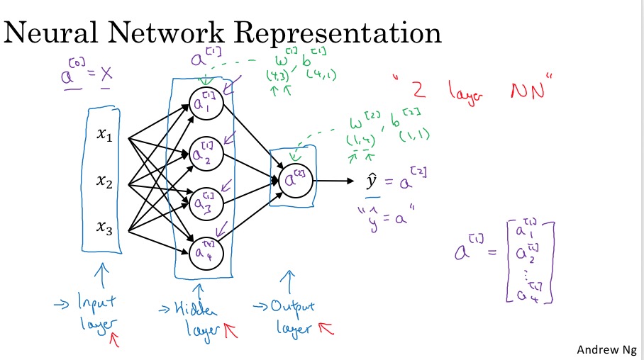
- Neural Network的组成:一个input layer,多个hidden layer,一个output layer
- training set作为输入层,即第0层,因此有 \(X = a^{[0]}\)
- 每一层输入,上标[i]表示layer的层数,下标j表示neuron的序号(每层有多个neuron)
- 一个惯例,input layer不计算在neuron Network的层数里,并且input layer的上标是0。因此一个例子中的是neural network是2层的。
- 注意每层的参数w和b的维度。w的行数是本层的neuron的个数,行数是上一层neuron的个数。b是一个列向量,行数与w相同。
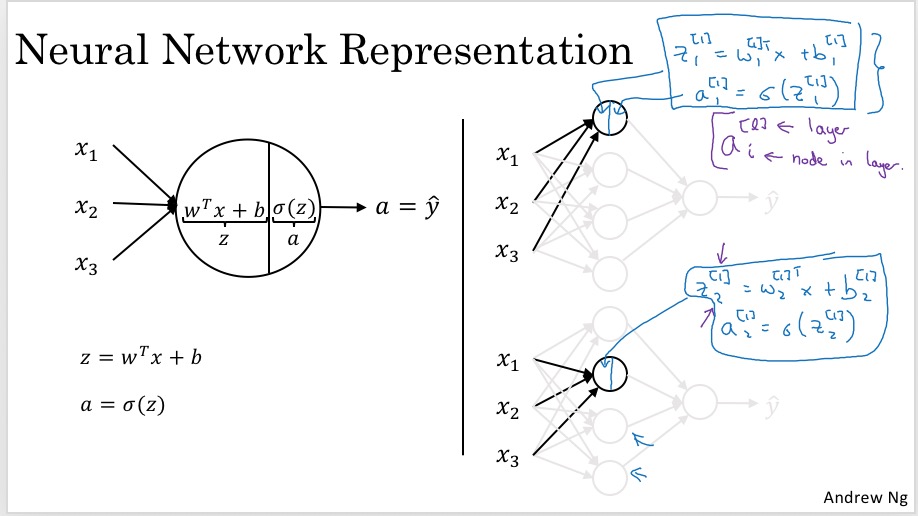
Computing a Neural Network’s Output
每个neuron的计算分为两步:z计算出线性组合,a计算激活函数:
每层的计算向量化(注意这里只是一个数据样本x的情况,后面会讲如何扩展为m个数据样本的情况):
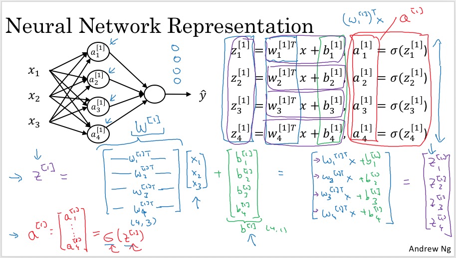
整理后,向量化的表示:
Given input x(a single training set):
\(z^{[1]} = W^{[1]}a^{[0]} + b^{[1]}\) \(a^{[1]} = \sigma(z^{[1]})\) \(z^{[2]} = W^{[2]}a^{[1]} + b^{[2]}\) \(a^{[2]} = \sigma(z^{[2]})\)
两点说明:
- 对中括号上标,本层的输出a,和参数w、b的上标是一样的,而输入的上标则是上一层的。有些文档里可能会把w、b的上标保持和上一层一样,这是不同的习惯吧。
- 上面计算时的\(w^{[1]}_1\)做了转置,最终向量化时W没有没有转置,这是因为前者是按照logistic regression的习惯定义的,即w是列向量。而后者是W的定义,每一行是该层对应neuron的参数,已经行向量了。
Vectorizing across multiple examples
前一节,已经强调了是针对一个training example的向量化,这一节要进一步对所有training example做向量化。
-
首先,是非向量化的实现,即对m个training example进行迭代如下:
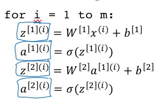 即在上一节的公式上,对x、z、a添加小括号上标。z和a和x的维度是一样的,即和training example对应的,而参数w和b没有training example这一维度,或者说w和b是对所有m个training example计算结果做平均。
 -
向量化
- 先弄清每个矩阵的维度X,Z以及A。三个变量的维度是一致的,在column方向都表示不同的training example;在row的方向表示不同的neuron:
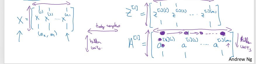
- 基于上面对X,Z以及A的定义,有: \(Z^{[1]} = W^{[1]}A^{[0]} + b^{[1]}\) \(A^{[1]} = \sigma(Z^{[1]})\) \(Z^{[2]} = W^{[2]}A^{[1]} + b^{[2]}\) \(A^{[2]} = \sigma(Z^{[2]})\)
- 先弄清每个矩阵的维度X,Z以及A。三个变量的维度是一致的,在column方向都表示不同的training example;在row的方向表示不同的neuron:
Explanation for Vectorized Implementation
其实就一句话:一个矩阵A乘以B,且B是列向量,那么B扩展为矩阵是没有问题的,结果也从一个列向量变成矩阵。
When you took the different training examples and stacked them up in different columns, then the corresponding result is that you end up with the z’s also stacked at the columns.
对于b来说,其实和X的个数无关,只要做broadcasting即可。
截止到上面,就是 (2 layer) Neural Network的forward propagation的向量化实现。
Activation functions
-
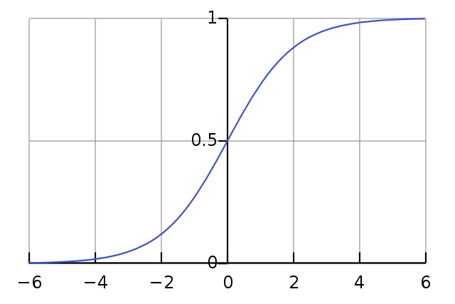
activation function是指将线性组合计算的z,进一步映射的non-linear function。比如sigmoid function就是将线性组合计算的z从实数域映射到了开区间(0,1)。
- 常用的activation function有:
-
sigmoid function \(a = \sigma(z) = \frac{1}{1+e^{-z}}\) 映射到开区间(0,1)
-
tanh function: a shift verison a sigmoid function \(a = tanh(z) = \frac{e^{z}-e^{-z}}{e^{z}+e^{-z}}\) 映射到开区间(-1,1)
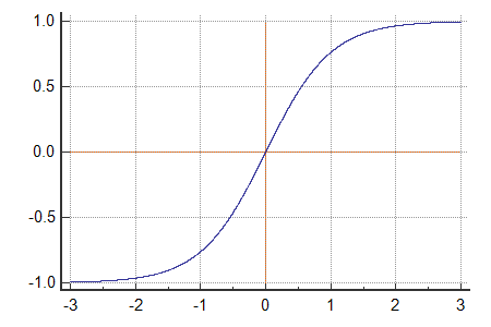 在hidden layer中用tanh代替sigmoid,基本上效果会更好,因为tanh会产生一个均值为0的结果,相当于自动做了中心化处理。
Andrew对选用sigmoid还是tanh的建议:hidden layer尽量用tanh而不是sigmoid,output layer根据输出需要可用sigmoid;另外每一层也可以选用不同的activation function。
在hidden layer中用tanh代替sigmoid,基本上效果会更好,因为tanh会产生一个均值为0的结果,相当于自动做了中心化处理。
Andrew对选用sigmoid还是tanh的建议:hidden layer尽量用tanh而不是sigmoid,output layer根据输出需要可用sigmoid;另外每一层也可以选用不同的activation function。 -
ReLU function \(a = max(0,a)\)
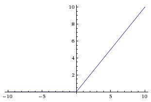 sigmoid和tanh共同的不足是:当z很大或很小时,导数都趋近于0,这会导致梯度下降的速度比较慢。因此,又引入了ReLU function(Rectified Linear Unit),这个名字听起来挺牛逼,但实际表达式很简单,就是将线性函数小于0的部分做了修正(Rectifed),最简单的修正就是直接让其等于0。
而且Andrew极力推荐ReLU:
sigmoid和tanh共同的不足是:当z很大或很小时,导数都趋近于0,这会导致梯度下降的速度比较慢。因此,又引入了ReLU function(Rectified Linear Unit),这个名字听起来挺牛逼,但实际表达式很简单,就是将线性函数小于0的部分做了修正(Rectifed),最简单的修正就是直接让其等于0。
而且Andrew极力推荐ReLU:if you’re not sure what to use for your hidden layer, I would just use the relu activation function that’s what you see most people using these days.
ReLU的一个好处是(我也不确定为什么是好处,Andrew只是说 in practice this works just fine):ReLU在小于0的时候,导数为0。 ReLU另一个版本叫做Leaky ReLU,即在小于0的部分,修正为一个斜率很小的直线(ReLU修正为了斜率为0的直线):
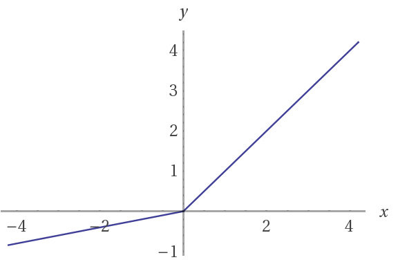 Leaky ReLUE通常比ReLU效果更好,但实践中去不常用(为毛好的东西不用?)。
相比sigmoid或tanh,ReLU或Leaky ReLU计算的更快 ,这也很显然,线性函数的导数就是一个常数。
Leaky ReLUE通常比ReLU效果更好,但实践中去不常用(为毛好的东西不用?)。
相比sigmoid或tanh,ReLU或Leaky ReLU计算的更快 ,这也很显然,线性函数的导数就是一个常数。 -
- Activation Function的建议
- sigmoid:除非在output layer要做binary classification会用到,hidden layer几乎不会用。要用也是有限用tanh
- 默认或最常用的是ReLU(或者也可以尝试Leaky ReLU)
- 面对具体情况,也可以尝试不同的算法,再选择最好的。
Why do you need non-linear activation functions?
一句话解释:
the composition of two linear functions is itself a linear function.
因此无论你做多少层的network,其实与做一层没什么区别。
当然,在output layer是可以不用activation function,或者用linear activation function;这种情况一般是要求输出实数集结果(比如预测房价)。即便如此,在hidden layer还是要用non-linear activation function。
Derivatives of activation functions
三种activation function的导数:
- sigmoid function \(\frac{d}{dz}\sigma(z) = \frac{d}{dz} \frac{1}{1+e^{-z}} = \sigma(z)(1 - \sigma(z))\) 推导参考: https://beckernick.github.io/sigmoid-derivative-neural-network/
- tanh function \(\frac{d}{dz}tanh(z)=1- tanh(z)^2\) 推导参考: http://math2.org/math/derivatives/more/hyperbolics.htm https://math.stackexchange.com/questions/741050/hyperbolic-functions-derivative-of-tanh-x
- ReLU function 这个就很简单了,唯一要注意0的时候不可导,因此做个修正,直接定义0点的导数为0。
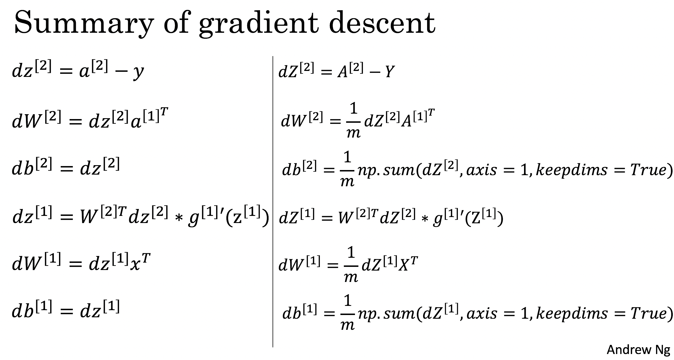
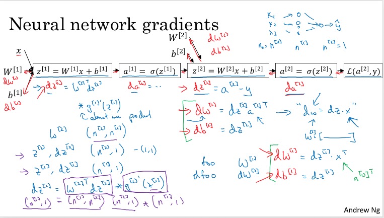
Gradient descent for Neural Networks
- gradient descent的关键是求cost function对参数的偏导数
- 求导过程使用的是Backpropagation
- 首先做forward propagation,求解出每一层的输出A
- 然后向后,逐层求解对每一层参数的偏导数
- 课程里并没有backpropagation的推导,只是给出了结果:
 Backpropagation具体推导过程,非常推荐这篇文章:How the backpropagation algorithm works
Backpropagation intuition (optional)
- 首先用logistic regression解释了backpropagation
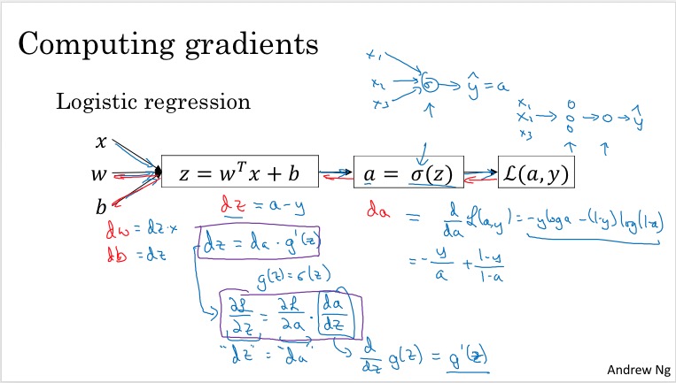
- 然后在2 layer Neuro Networks上解释
Random Initialization
与logistic regression不同,初始化参数不可固定为0,而是每个参数都要随机初始化。
主要原因是:如果每个参数w和b都是0,则同一层的每个neuron计算结果完全一样(输入一样a,参数一样w,则z一样);接下来反向传播时的偏导数也一样,下一轮迭代同一层的每个neuron的w又是一样的。这样整个neural Network上每一层的neuron是同质的,自然不会有好的performance。
不过,对b参数,可以都初始化为0。
另外需要注意,虽然w是随机初始化,但最好使用较小的随机数。主要是避免让z的计算值过大,导致activation function对z的偏导数趋于0,导致Gradient descent下降较慢。 通常的做法是对random的值乘以一个比率,比如0.01(但具体怎么选这个比率,也要根据情况而定,这应该又是一个超参了): \(W^{[1]} = np.random.randn((2,2)) * 0.01\)
The general methodology to build a Neural Network is to:
- Define the neural network structure ( # of input units, # of hidden units, etc).
- Initialize the model’s parameters
- Loop:
- Implement forward propagation
- Compute loss
- Implement backward propagation to get the gradients
- Update parameters (gradient descent)
Heros of Deep learning: Ian Goodfellow interview

- 这位就是大名鼎鼎的花书Deep Learning的作者,原以为是个白胡子老头,没想到竟然是个85后。
- 学习了Andrew Ng 的 Machine Learning 开始对AI感兴趣。
I started to have a very strong intuition that deep learning was the way to go in the future.
- How did you come up with GANs (Generative Adversarial Networks)?
- GANs 可以自动生成更多的训练数据。
- GANs were introduced in a paper by Ian Goodfellow and other researchers at the University of Montreal, including Yoshua Bengio, in 2014.
-
I implemented it around midnight after going home from the bar where my friend had his going-away party.
- 有一次人都差点挂了,第一想到的还是怎么把自己的研究尽快弄出来。
- 和自己的两个 Ph.D. 导师共同编写了Deep Learning这本书。
- 特别提到了中文版和英文版卖的都很好。
- 与其他书不同,本书中特别介绍了 Deep Learning 需要的数学知识。
-
If you want to be a really excellent practitioner, you’ve got to master the basic math that underlies the whole approach in the first place.
-
And now, we’re at a point where there are so many different paths open that someone who wants to get involved in AI, maybe the hardest problem they face is choosing which path they want to go down.
- Advice for someone wanting to get into AI.
- Ph.D. is not a absolute requirement any more.
- One way that you could get a lot of attention is to write good code and put it on GitHub.
- I think if you learned by reading the book, it’s really important to also work on a project at the same time.
- Work on adversarial examples.
- It’s a new field called machine learning security.
(另外,这家伙居然几乎不眨眼,也不转动眼球。)
系列笔记:deeplearning.ai深度学习笔记系列首页
-------------------------
本文采用 知识共享署名 4.0 国际许可协议(CC-BY 4.0)进行许可。转载请注明来源:https://imshuai.com/deeplearning-ai-notes-course1-week3 欢迎指正或在下方评论。
毛帅
{Code, Thoughts, Sharing}