deeplearning.ai深度学习笔记(Course2 Week3):Hyperparameter tuning, Batch Normalization and Programming Frameworks
本周介绍了深度学习超参的调优方法,Batch Norm算法、Softmax实现多元分类。并以tensorflow介绍了deep learing框架。
1- Hyperparameter tuning
1.1- Turning process
- 到目前为止,我们接触到的hyperparameter有:
- learning rate: \(\alpha\)
- momentum 参数: \(\beta\)
- Adam参数: \(\beta_1\)和 \(\beta_2\)以及\(\varepsilon\)
- 神经网络层数: L
- 神经网络隐藏层neuron数:\(n^{[l]}\)
- learning rate decay参数
- min-batch size
- 这些hyperparameter重要性排序:
- 最重要的: learning rate: \(\alpha\)
- 比较重要的: momentum 参数: \(\beta\) 神经网络层数: L 神经网络隐藏层neuron数:\(n^{[l]}\)
- 次重要的: 神经网络隐藏层neuron数 learning rate decay参数
- 基本不需调整的 \(\beta_1\)和 \(\beta_2\)以及\(\varepsilon\)
- 如何搜索hyperparameter
- 使用随机搜索,而不是在网格中定点搜索
- 先整体粗略搜索,再到表现好的区域精细搜索。
1.2- Using an appropriate scale to pick hyperparameters
上面虽然说是“随机”搜索,但不是完全的随机,而是在合理的范围内搜索,同时在范围内搜索,也不是均匀分布(uniformly random)的,通常有这个参数的scale,比如对数scale。
比如α,一般是使用log scale。比如α的合理区间是[0.0001, 1],并不是说在这个区间随机的进行均匀分布的搜索,手工选择是会这样:先选择0.0001,不好的话再选择0.001,0.01等, 这是因为对于learning rate来说,线性scale并不敏感。
放到Python中实现是:
r = -4 * np.random.rand()  # r取值范围是[-4,1]的均匀分布
α = 10^r
这个做法的结果是α的对数满足均匀分布。
又比如β的合理区间是0.9到0.999。β取值0.9和0.905的区别很小,相当于取最近10个或10.5个均值的差异。但同样增加0.005,0.994和0.999就截然不同,前者相当于对最近200个数值的加权平均,而后者相当于最近1000个数值的加权平均。
可以这样实现:
r = -2 * np.random.rand() -1 # r取值在[-3,-1]的均匀分布
1-β = 10^r
β = 1 - 10^r
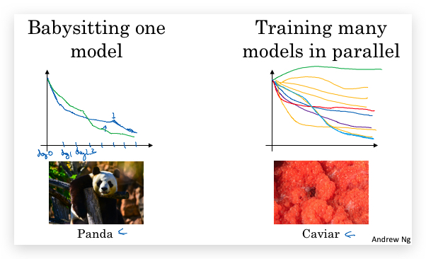
1.3- Hyperparameters tuning in practice: Pandas vs. Caviar
- 不同的算法和场景,对超参的scale敏感性可能不一样.
- 根据计算资源和数据量,可以采取两种策略来调参
- Panda(熊猫策略):对一个模型先后修改参数,查看其表现,最终选择最好的参数。就像熊猫一样,一次只抚养一个后代。
- Caviar(鱼子酱策略):计算资源足够,可以同时运行很多模型实例,采用不同的参数,然后最终选择一个好的。类似鱼类,一次下很多卵,自动竞争成活。
2- Batch Normalization
2.1- Normalizing activations in a network
- 基本思想: 在机器学习算法中,我们会将输入数据X做 Normalization 处理,使得每个属性都在同一个尺度上,从而加快梯度下降的速度。同样在深度学习网络中,也会对输入数据X做 Normalization 处理,但网络中有隐藏层,隐藏层内的输入是上一层的输出,同样面临隐藏层的输入数据不在同一尺度上的问题。 因此最简单的办法是对每一层的输入,即上一层activation function的输出做normalization。
2.Batch Norm的实现 实践中,是对z进行normalization,具体算如下: 对某一层l的中间值\(Z^{[l]}\)(注意下面的计算都是向量,计算都省略了上标l), 先计算均值和方差: \(\mu = \frac{1}{m} \sum_i z^{(i)}\) \(\sigma^2 = \frac{1}{m} \sum_i {(z^{(i)} - \mu)}^2\) 然后对每一个样本i的z进行标准化(分母增加\(\varepsilon\)是为了防止方差为0,一般取10^-8): \(z_{norm}^{(i)} = \frac{z^{(i)} - \mu}{\sqrt{\sigma^2 + \varepsilon}}\)
-
从normalization的目的看,已经完成了。但实际上在深度网络中,我们希望每一层拥有不同的分布(即不同的\( \mu \)和\(\sigma^2\)),尤其是对于sigmoid等activation function来说,z如果处于均值为0,方差为1的范围,无法充分利用到activation function的non-linear特性,因为在这范围,sigmoid函数近似的表现为线性函数。因此会再次处理: \(\tilde z^{(i)} = \gamma z^{(i)}\_{norm} + \beta\) 处理后,\(\tilde z^{(i)} \)将服从均值为\(\beta \),方差为\(\gamma\)的分布。 需要注意的是,\(\beta \)和\(\gamma\)不是超参,而是梯度下降需学习的参数。
-
接下来,用\(\tilde z^{(i)} \)代替\(z^{(i)} \)输入到activation function计算。
2.2- Fitting Batch Norm into a neural network
上面讲的是如何将batch norm应用到一层网络中,下面将介绍如何将batch norm应用到整个网络中。 实际上就是在z和a的计算中间增加了一道BN(Batch Norm):
\[X \xrightarrow{W^{[1]},b^{[1]}} Z^{[1]} \xrightarrow[BN]{\beta^{[1]},\gamma^{[1]} } \tilde Z^{[1]} \xrightarrow{g^{[1]}} A^{[1]} \xrightarrow{} ... A^{[L-1]} \xrightarrow{W^{[L]},b^{[L]}} Z^{[L]} \xrightarrow[BN]{\beta^{[L]},\gamma^{[L]} } \tilde Z^{[L]} \xrightarrow{g^{[L]}} A^{[L]}\]从梯度下降算法上看,和W和b的地位是一样的了,也是需要学习的参数了。
由于β会再次对Z设置均值,因此原来的bias参数b就可以省略了(作用其实和β重复了),所以在应用batch-norm的情况下,参数b就省略了,实际要训练的参数只有W,β和γ,对应的流程如下: \(X \xrightarrow{W^{[1]}} Z^{[1]} \xrightarrow[BN]{\beta^{[1]},\gamma^{[1]} } \tilde Z^{[1]} \xrightarrow{g^{[1]}} A^{[1]} \xrightarrow{} ... A^{[L-1]} \xrightarrow{W^{[L]}} Z^{[L]} \xrightarrow[BN]{\beta^{[L]},\gamma^{[L]} } \tilde Z^{[L]} \xrightarrow{g^{[L]}} A^{[L]}\)
其中对每一层的\(\beta^{[l]}\)与\(\gamma^{[l]}\)的shape都和\(Z^{[l]}\)一样,都是\((n^{[x]},1)\)。
伪代码实现:
for t =1,num of mini batch:
    compute forward prop on X^{t}
        in each hidden layer, use BN to replace Z^[l]
    use backprop to compute dW^[l], dβ^[l], dγ^[l]
    update parameters
        W^[l] -= α * dW^[l]
        β^[l] -= α * dβ^[l]
        γ^[l] -= α * dγ^[l]
这种batch-norm改进过的梯度下降算法,同样可以使用前面学过的mini-batch、momentum、RMSprop和Adam。
2.3- Why does Batch Norm work?
Batch Norm总体上有三个作用:
- 首先,起到了normalization的作用,同对输入数据X的normalization作用类似。
- 让每一层的学习,一定程度解耦了前层参数和后层参数,让各层更加独立的学习。无论前一层如何变,本层输入的数据总是保持稳定的均值和方差。(主要原因)
- 有轻微的regularization effect(虽然不是BN算法的本意,尽是顺带的副作用)。 对于min-batch来说,每一个mini-batch采用的mean/variance不一样,相当于对z的计算引入了一定的噪声,类似于dropout算法,对a的计算引入了噪声,让下游的hidden units不过度依赖于上层的某个hidden unit。mini-batch的size越大,regularization effect越小。
关于第二点,Batch norm使得后层的hidden layer比初始数据更具鲁棒性。数据样本的变化(比如原本都是黑猫,现在增加了彩色猫),可能导致数据的分布随着变化,即Covariate Shift(协变量),就需要重新训练学习算法,And this is true even if the function, the ground true function, mapping from X to Y, remains unchanged, which it is in this example, because the ground true function is, is this picture a cat or not.
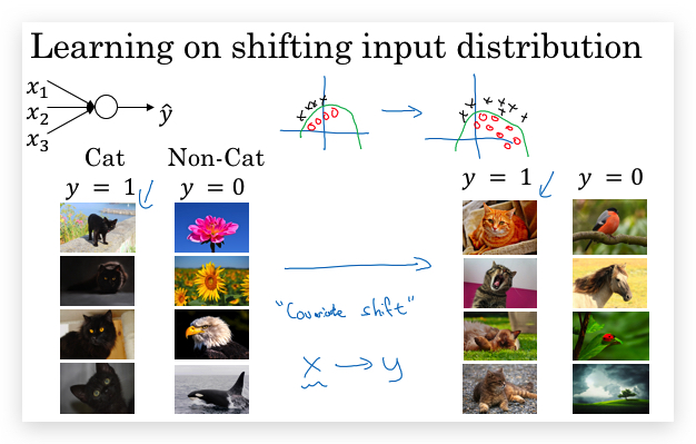
What batch norm does, is it reduces the amount that the distribution of these hidden unit values shifts around。BN算法限制了输入数据的变化对当前层依赖的隐藏层输入的分布影响。
2.4- Batch Norm at test time
问题:BN算法在训练时是一个批次的数据训练,能算出每一层Z的均值和方差;而在测试时,输入的则是单个数据,单条数据没法做均值和方差的计算,怎么在测试期输入均值和方差呢?
思路:在training阶段,就通过exponentially weighted average的方法,顺便计算μ和σ^2针对每一个epoch的加权平均。 最终用迭代完成后的这个加权平均作为test阶段的μ和σ^2
理论上,还有一种思路:可以在迭代结束后,做一次全量测试数据X的forward propagation,在每一层计算μ和σ^2,用作test阶段的μ和σ^2,实践中更多的用上面的思路。
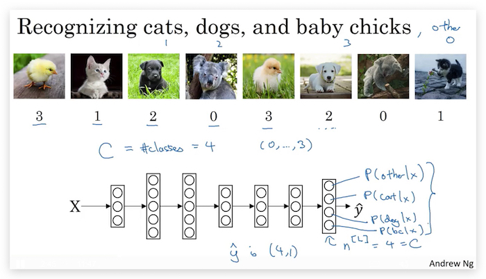
3- Multi-class classification
问题:之前的Neural Network都是二元分类,比如识别是否是猫咪。如果要识别的类别多余两个,比如要识别图中的动物是(猫, 小鸡, 狗, 其他)则称为Multi-class classification。下面将介绍如何处理。
3.1- Softmax Regression
假设要分类的个数记为\(C\)(比如上例中\(C=4\)) 首先,在设计网络时,让最后一层的neuron个数为\(n^{[L]}=C\),每一个neuron输出每一个class的概率,如下图:
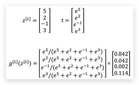
为了实现上面的设计,对最后一层使用Softmax Layer。 实现softmarx Layer的关键是activation function改为如下计算方法: 计算\(z^{[L]}\)的算法不变,计算\(a^{[L]}\)的算法如下: 先对\(z^{[L]}\)取自然对数为底的指数(注意t是向量): \(t = \mathrm{e}^{(z^{[L]})}\) 然后计算\(a^{[L]}\): \(a^{[L]} = \frac{t}{\sum\limits_{j = 1}^{C}t_j}\)
在这种计算下,a值有特性: \(\sum^C_{i=1}a^{[L]}_i = 1\)
具体来说,就是将每个neuron的z做e的指数,然后用这个结果的占比作为a。
举例:
 对于soft layer的activation function要注意一点:虽然看起来输入是向量,输出的也是向量,但与sigmoid或tanh等不一样。后者,只是vectorization的结果,实际每个neuron的activation计算是相互独立,互不影响的。但对于soft layer,并不相互独立,输入是整个\(z^{[L]}\)因为中间需要对所有的t进行加总,因此任何一个neuron的z值改变,都会影响所有neuron的a值。
疑问:
- 为什么要做e的指数?
- 和one-vs-all比较,有什么优势?
参考资料:Softmax回归-ufldl
3.2- Training a softmax classifier
- Understanding softmax
- 对比hard max
- Softmax regression将logistic regression推广到C个分类。如果C=2,softmax则退化为logistic regression。
-
Loss function 与logistic regression一样,也是取对数: \(L(\hat y, y) = -\sum^C_{j=1}y_j\log\hat y_j\) 虽然这是一个求和,但实际对应到一个样本时,只会有一个\(y_j\)等于1,其他的都是0,假如是第t个为1,则有: \(L(\hat y, y) = -\log\hat y_t\) 若让L最小,显然就是让\(\hat y_t \)最大,即让和数据集实际值匹配的y的概率最大。Logistics Regression的Loss function可以看成其特例。
-
Cost Function 很简单,就素对的所有Loss function求均值。 \(J(W, b, ...) = \frac{1}{m} \sum^m_{i=1}L(\hat y^{(i)}, y^{(i)})\)
- Gradient descent with softmax 与原来的Gradient descent的主要区别是backprop时计算最后一层对Z的偏导数\(dz^{[L]}\) : \(dz^{[L]} = \hat y- y\)
4- Introducton to programming frameworks
4.1- Deep learning frameworks
之前我们都是从头自己写算法(from scratch),接下来我们在了解原理的基础上,没必要去实现复杂的细节了。
Deep learning framewroks:
- Caffe/Caffe2
- CNTK
- DL4J
- Keras
- Lasagne
- mxnet
- PaddlePaddle
- TensorFlow
- Theano
- Torch
Choosing deep learning frameworks
- Ease of programming (development and deployment)
- Running speed
- Truly open (open source with good governance)
4.2- TensorFlow
- 以一元二次函数为例,计算下面的cost function的最小值对应的参数w:
import numpy as np
import tensorflow as tf # 导入Tensorflow

w = tf.Variable(0, dtype=tf.float32)
cost = w**2 - 10*w + 25 # 要优化的cost function(即forward prop的形式)
train = tf.train.GradientDescentOptimizer(0.01).minimize(cost)

init = tf.global_variables_initializer()
session = tf.Session()
session.run(init)
print(session.run(w))

session.run(train)
print(session.run(w))

for i in range(1000):
    session.run(train)
print(session.run(w))
使用tensorflow,只要告诉tensorflow forward prop,它自己就会做backprop,因此不用自己实现backprop
- placeholder 在实际的训练过程中,要用不同的样本反复放到一个待优化函数中的,这个时候就可以用tensorflow的placeholder实现。举例如下:
import numpy as np
import tensorflow as tf # 导入Tensorflow

coefficient = np.array([[2.],[-10.],[25.]])

w = tf.Variable(0, dtype=tf.float32)
x = tf.placeholder(tf.float32, [3,1]) # 3x1大小的placeholder
cost = w**x[0][0] - x[1][0]*w + x[2][0] # 要优化的cost function(即forward prop的形式)
train = tf.train.GradientDescentOptimizer(0.01).minimize(cost)

init = tf.global_variables_initializer()
session = tf.Session()
session.run(init)
print(session.run(w))

session.run(train, feed_dict={x:coefficient}) # x占位符替换为coefficient
print(session.run(w))

for i in range(1000):
    session.run(train, feed_dict={x:coefficient}) # # x占位符替换为coefficient
print(session.run(w))
使用tf.placeholder(tf.float32, [3,1])构造了一个3x1大小的placeholder,然后输入到cost函数cost = w**x[0][0] - x[1][0]*w + x[2][0],在run的时候,对应给出feed_dict,表名占位符x的实际值。
- with语句
为了自动回收session,可以用Python的with语句声明session对象:
with tf.Session() as session: session.run(init) print(session.run(w)) - computation graph
上面的例子
cost = w**x[0][0] - x[1][0]*w + x[2][0]实际是告诉tensorflow如何生成计算图,进而可以做forward prop和backprop
5- TensorFlow作业
以下内容从本周的作业总结:
- Writing and running programs in TensorFlow has the following steps:
- Create Tensors (variables) that are not yet executed/evaluated.
- Write operations between those Tensors.
- Initialize your Tensors.
- Create a Session.
- Run the Session. This will run the operations you’d written above.
- 理解run Therefore, when we created a variable for the loss, we simply defined the loss as a function of other quantities, but did not evaluate its value. To evaluate it, we had to run init=tf.global_variables_initializer(). That initialized the loss variable, and in the last line we were finally able to evaluate the value of loss and print its value.
tf中的运算只是定义operation,添加到了运算图,但实际运算还没有进行;实际运算是靠session.run方法完成的。 一个简单的例子:
a = tf.constant(2)
b = tf.constant(10)
c = tf.multiply(a,b)
print(c) # 输出 Tensor("Mul:0", shape=(), dtype=int32)
上面tf.multiply并不会立即计算出c的值,print(c)的结果只是一个空白的tensor。
接下来,创建session,然后run(c),才会有结果:
sess = tf.Session()
print(sess.run(c)) # 输出 20
- place holder
A placeholder is simply a variable that you will assign data to only later, when running the session. We say that you feed data to these placeholders when running the session. 举例:
# Change the value of x in the feed_dict
x = tf.placeholder(tf.int64, name = 'x')
print(sess.run(2 * x, feed_dict = {x: 3}))
sess.close() # 输出 6
Here’s what’s happening: When you specify the operations needed for a computation, you are telling TensorFlow how to construct a computation graph. The computation graph can have some placeholders whose values you will specify only later. Finally, when you run the session, you are telling TensorFlow to execute the computation graph.
- 最后作业给出了一个tensorflow的框架代码,很有参考意义,这里收藏一下,供以后参考:
def model(X_train, Y_train, X_test, Y_test, learning_rate = 0.0001,
       num_epochs = 1500, minibatch_size = 32, print_cost = True):
 """
 Implements a three-layer tensorflow neural network: LINEAR->RELU->LINEAR->RELU->LINEAR->SOFTMAX.

 Arguments:
 X_train -- training set, of shape (input size = 12288, number of training examples = 1080)
 Y_train -- test set, of shape (output size = 6, number of training examples = 1080)
 X_test -- training set, of shape (input size = 12288, number of training examples = 120)
 Y_test -- test set, of shape (output size = 6, number of test examples = 120)
 learning_rate -- learning rate of the optimization
 num_epochs -- number of epochs of the optimization loop
 minibatch_size -- size of a minibatch
 print_cost -- True to print the cost every 100 epochs

 Returns:
 parameters -- parameters learnt by the model. They can then be used to predict.
 """

 ops.reset_default_graph()                         # to be able to rerun the model without overwriting tf variables
 tf.set_random_seed(1)                             # to keep consistent results
 seed = 3                                          # to keep consistent results
 (n_x, m) = X_train.shape                          # (n_x: input size, m : number of examples in the train set)
 n_y = Y_train.shape[0]                            # n_y : output size
 costs = []                                        # To keep track of the cost

 # Create Placeholders of shape (n_x, n_y)
 ### START CODE HERE ### (1 line)
 X, Y = create_placeholders(n_x, n_y)
 ### END CODE HERE ###

 # Initialize parameters
 ### START CODE HERE ### (1 line)
 parameters = initialize_parameters()
 ### END CODE HERE ###

 # Forward propagation: Build the forward propagation in the tensorflow graph
 ### START CODE HERE ### (1 line)
 Z3 = forward_propagation(X, parameters)
 ### END CODE HERE ###

 # Cost function: Add cost function to tensorflow graph
 ### START CODE HERE ### (1 line)
 cost = compute_cost(Z3, Y)
 ### END CODE HERE ###

 # Backpropagation: Define the tensorflow optimizer. Use an AdamOptimizer.
 ### START CODE HERE ### (1 line)
 optimizer = tf.train.AdamOptimizer(learning_rate=learning_rate).minimize(cost)
 ### END CODE HERE ###

 # Initialize all the variables
 init = tf.global_variables_initializer()

 # Start the session to compute the tensorflow graph
 with tf.Session() as sess:

     # Run the initialization
     sess.run(init)

     # Do the training loop
     for epoch in range(num_epochs):

         epoch_cost = 0.                       # Defines a cost related to an epoch
         num_minibatches = int(m / minibatch_size) # number of minibatches of size minibatch_size in the train set
         seed = seed + 1
         minibatches = random_mini_batches(X_train, Y_train, minibatch_size, seed)

         for minibatch in minibatches:

             # Select a minibatch
             (minibatch_X, minibatch_Y) = minibatch

             # IMPORTANT: The line that runs the graph on a minibatch.
             # Run the session to execute the "optimizer" and the "cost", the feedict should contain a minibatch for (X,Y).
             ### START CODE HERE ### (1 line)
             _ , minibatch_cost = sess.run([optimizer, cost], feed_dict={X:minibatch_X, Y:minibatch_Y})
             ### END CODE HERE ###

             epoch_cost += minibatch_cost / num_minibatches

         # Print the cost every epoch
         if print_cost == True and epoch % 100 == 0:
             print ("Cost after epoch %i: %f" % (epoch, epoch_cost))
         if print_cost == True and epoch % 5 == 0:
             costs.append(epoch_cost)

     # plot the cost
     plt.plot(np.squeeze(costs))
     plt.ylabel('cost')
     plt.xlabel('iterations (per tens)')
     plt.title("Learning rate =" + str(learning_rate))
     plt.show()

     # lets save the parameters in a variable
     parameters = sess.run(parameters)
     print ("Parameters have been trained!")

     # Calculate the correct predictions
     correct_prediction = tf.equal(tf.argmax(Z3), tf.argmax(Y))

     # Calculate accuracy on the test set
     accuracy = tf.reduce_mean(tf.cast(correct_prediction, "float"))

     print ("Train Accuracy:", accuracy.eval({X: X_train, Y: Y_train}))
     print ("Test Accuracy:", accuracy.eval({X: X_test, Y: Y_test}))

     return parameters
另外,这个方法在Coursera的jupyter notebook似乎训练很慢,并不像作业里面提示的5min完成,我估计了一下至少要1500s
-------------------------
本文采用 知识共享署名 4.0 国际许可协议(CC-BY 4.0)进行许可。转载请注明来源:https://imshuai.com/deeplearning-ai-notes-course2-week3 欢迎指正或在下方评论。
毛帅
{Code, Thoughts, Sharing}